

Tracking technology has been a part of football analysis for the past 20 years, giving access to data on physical performance and heat map visualisations that show how far and wide a player covers. As this technology becomes cheaper and more accessible, it has now become easy for anyone to get this data on their Sunday morning games. This article runs through how you can create your own heatmaps for a game, with nothing more than a GPS tracking device (running watch, phone, gps unit) and Python.
To get your hands on your own data, you can extract your gpx file through Strava. While Strava is great for runs, it isn’t built for football or running in tight spaces. So let’s build our own!
Let’s import our necessary modules and data, then get started!
#GPXPY makes using .gpx files really easy
import gpxpy

#Visualisation libraries
import matplotlib.pyplot as plt
%matplotlib inline
import seaborn as sns

#Opens our .gpx file, then parses it into a format that is easy for us to run through
gpx_file = open('5aside.gpx', 'r')
gpx = gpxpy.parse(gpx_file)
The .gpx file type, put simply, is a markup file that records the time and your location on each line. With location and time, we can calculate distance between locations and, subsequently, speed. We can also visualise this data, as we’ll show here.
Let’s take a look at what one of these lines looks like:
gpx.tracks[0].segments[0].points[0]
The first two points are our latitude and longitude, alongside elevation and time. This gives us a lot of freedom to calculate variables and plot our data, and is the foundation of a lot of the advanced metrics that you will find on Strava.
In our example, we want to plot our latitude and longitude, so let’s use a for loop to add these to a list:
lat = []
lon = []

for track in gpx.tracks:
    for segment in track.segments:
        for point in segment.points:
            lat.append(point.latitude)
            lon.append(point.longitude)
Our location is now extraceted into a handy x and y format….let’s plot it. We’ve borrowed Andy Kee‘s Strava plotting aesthetic here, take a read of his article for more information on plotting your cycle/run data!
fig = plt.figure(facecolor = '0.1')
ax = plt.Axes(fig, [0., 0., 1., 1.], )
ax.set_aspect('equal')
ax.set_axis_off()
fig.add_axes(ax)
plt.plot(lon, lat, color = 'deepskyblue', lw = 0.3, alpha = 0.9)
plt.show()

The lines are great, and make for a beautiful plot, but let’s try and create a Prozone-esque heatmap on our pitch.
To do this, we can plot on the actual pitch that we played on, using the gmplot module. GM stands for Google Maps, and will import its functionality for our plot. Let’s take a look at how this works:
#Import the module first
import gmplot

#Start an instance of our map, with three arguments: lat/lon centre point of map - in this case,
#We'll use the first location in our data. The last argument is the default zoom level of the map
gmap = gmplot.GoogleMapPlotter(lat[0], lon[0], 20)

#Create our heatmap using our lat/lon lists for x and y coordinates
gmap.heatmap(lat, lon)

#Draw our map and save it to the html file named in the argument
gmap.draw("Player1.html")
This code will spit out a html file, that we can then open to get our heatmap plotted on a Google Maps background. Something like the below:
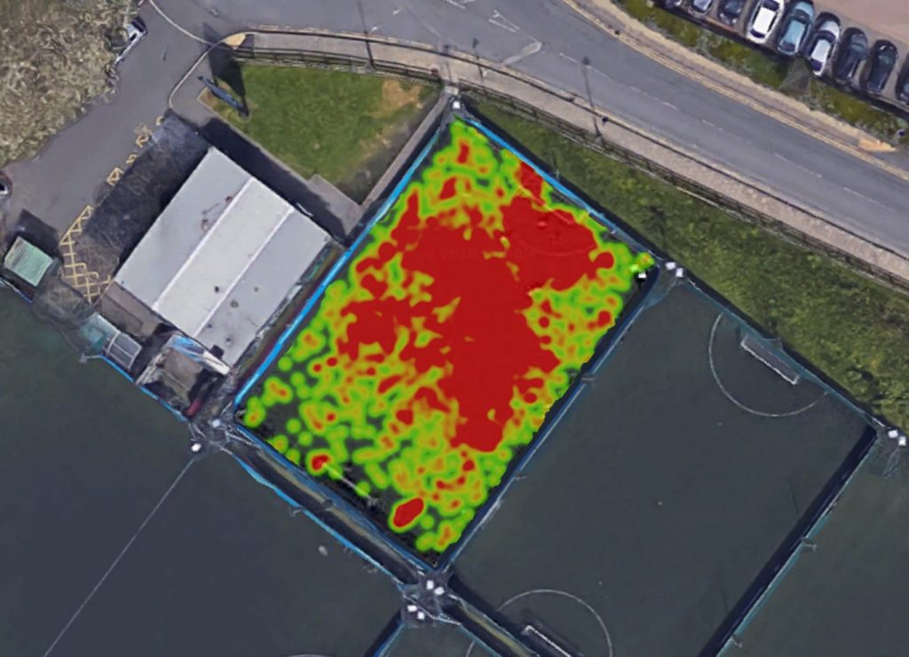
Summary
Similar visualisations of professional football matches set clubs and leagues back a pretty penny, and you can do this with entirely free software and increasingly affordable kit. While this won’t improve FC Python’s exceedingly poor on-pitch performances, we definitely think it is pretty cool!
Simply export your gpx data from Strava and extract the lat/long data, before plotting it as a line or as a heatmap on a map background for some really engaging visualisation.
Next up, learn about plotting this on a pitchmap, rather than satellite imagery.