

Working in Python, your data is likely to come from a number of different places – spreadsheets, databases or elsewhere. Eventually, you will find that some interesting and useful data for you will be available through a web API – a stream of data that you will need to call from, download and format for your analysis.
This article will introduce calling an API with the requests library, before formatting it into a dataframe and visualising it. Our example makes use of the fantastic work done at clubelo.com – a site that applies the elo rating system to football. Their API is easy to use and provides us with a great opportunity to learn about the processes in this article!
Let’s get our modules together and get started:
import requests
import csv
from io import StringIO
import pandas as pd
from datetime import datetime

import matplotlib.pyplot as plt
import seaborn as sns
Calling an API
Downloading a dataset through an API must be complicated, surely? Of course, Python and its libraries make this as simple as possible. The requests library will do this quickly and easily with the ‘.get’ function. All we need to do is provide the api location that we want to read from. Other APIs will require authentification, but for now, we just need to provide the API address.
r = requests.get('http://api.clubelo.com/ManCity')
If you would like to run the tutorial with a different team, take a look at the instructions here and find your club on the site to find the correct name to use.
Our new ‘r’ variable contains a lot of information. It will hold the data that we will analyse, the address that we called from and a status code to let us know if it worked or not. Let’s check our status code:
r.status_code
There are dozens of status codes, which you can find here, but we are hoping for a 200 code, telling us that the call went through as planned.
Now that we know that our request has made its way back, let’s check out what the API gives us with .text applied to the request (we have shortened the export dramatically, but it carries on as you see below):
r.text
We’re given a load of text that, if you read carefully, is separated by commas and ‘\n’. Hopefully you recognise that this could be a CSV file!
Formatting our request data
We need to turn this into a spreadsheet-style dataframe in order to do anything with it. We will do this in two steps, firstly assigning this text to a readable csv variable with the StringIO library. We can then use Pandas to turn it into a dataframe. Check out how below:
data = StringIO(r.text)
df = pd.read_csv(data, sep=",")

df.head()
Awesome, we have a dataframe that we can analyse and visualise! One more thing that we need to format are the date columns. By default, they are strings of text and we need to reformat them to utilise the date functionality in our analysis.
Pandas makes this easy with the .to_datetime() function. Let’s reassign the from and to columns with this:
df.From = pd.to_datetime(df['From'])
df.To = pd.to_datetime(df['To'])
Visualising the data
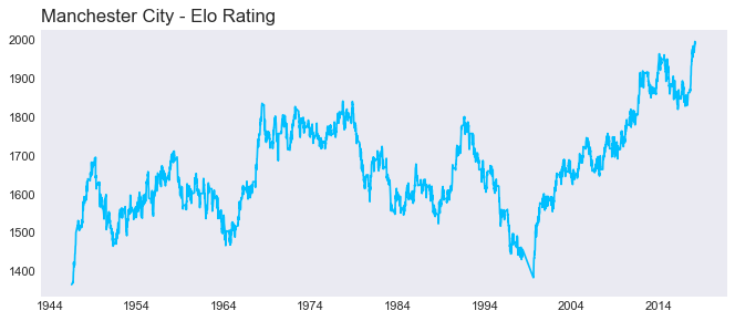
The most obvious visualisation of this data is the journey that a team’s elo rating has taken.
As we have created our date columns, we can use matplotlib’s plot_date to easily create a time series chart. Let’s fire one off with our data that we’ve already set up:
#Set the visual style of the chart with Seaborn Set the size of our chart with matplotlib
sns.set_style("dark")
plt.figure(num=None, figsize=(10, 4), dpi=80)

#Plot the elo column along the from dates, as a line ("-"), and in City's colour
plt.plot_date(df.From, df.Elo,'-', color="deepskyblue")

#Set a title, write it on the left hand side
plt.title("Manchester City - Elo Rating", loc="left", fontsize=15)

#Display the chart
plt.show()
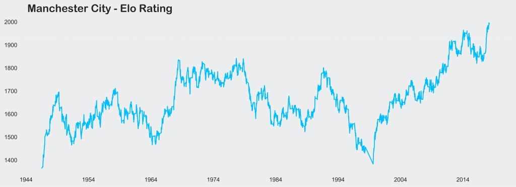
And let’s change a couple of the style options with matplotlib to tidy this up a bit. Hopefully you can figure out how we have changed the background colour, text style and size by reading through the two pieces of code.
#Set the visual style of the chart with Seaborn Set the size of our chart with matplotlib
sns.set_style("dark")
fig = plt.figure(num=None, figsize=(15, 5), dpi=600)
axes = fig.add_subplot(1, 1, 1, facecolor='#edeeef')
fig.patch.set_facecolor('#edeeef')


#Plot the elo column along the from dates, as a line ("-"), and in City's colour
plt.plot_date(df.From, df.Elo,'-', color="deepskyblue")

#Set a title, write it on the left hand side
plt.title("   Manchester City - Elo Rating", loc="left", fontsize=18, fontname="Arial Rounded MT Bold")

#Display the chart
plt.show()
Now this is a lot of code to piece through and do group-by-group, so let’s create a function to do it all in one go. Try and read through it carefully, matching it to the steps above.
def plotClub(team, colour = "dimgray"):
    r = requests.get('http://api.clubelo.com/' + str(team))
    data = StringIO(r.text)
    df = pd.read_csv(data, sep=",")

    df.From = pd.to_datetime(df['From'])
    df.To = pd.to_datetime(df['To'])

    sns.set_style("dark")
    fig = plt.figure(num=None, figsize=(12, 4), dpi=600)
    axes = fig.add_subplot(1, 1, 1, facecolor='#edeeef')
    fig.patch.set_facecolor('#edeeef')
    plt.plot_date(df.From, df.Elo,'-', color = colour)
    plt.title("    " + str(team) + " - Elo Rating", loc="left",  fontsize=18, fontname="Arial Rounded MT Bold")
    plt.show()
And let’s give it a go…
plotClub("RBLeipzig", "red")
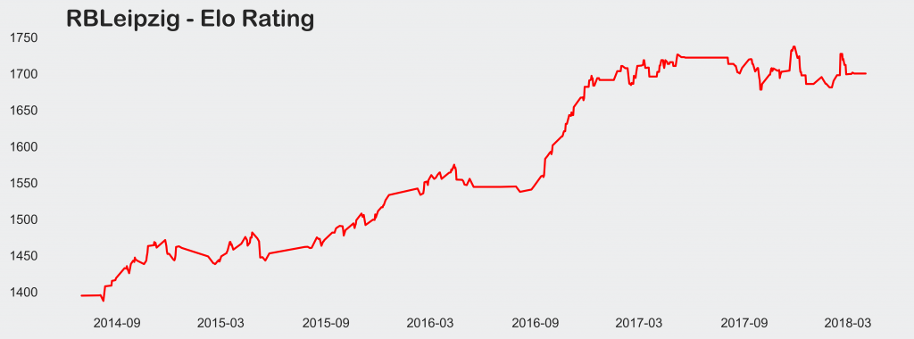
So we’re now calling, tidying and plotting our request in one go! Great work! Can you create a plot that compares two teams? Take a look through the matplotlib documentation to learn more about customising these plots too!
Of course, repeatedly calling an API is bad practice, so perhaps work on calling the data and storing it locally instead of making the same request over and over.
Summary
Being able to call data and structure it for analysis is a crucial skill to pick up and develop. This article has introduced the topic with the readily available and easy-to-utilise API available from clubelo. We owe them a thank you for their help and permission in putting this piece together!
To develop here, you should work on calling from APIs and storing the data for later use in a user-friendly format. Take a look at other sport and non-sport APIs and get practicing!
If you would like to learn more about formatting our charts like we have done above, take a look through some rules and code for better visualisations in Python.