

2020 is a Euros year, and guaranteed THE year that England end x years of hurt.
Of course, it will not be plain sailing and I’m sure that there will be ups and downs along the way. To console and to celebrate, we need the England classics as the soundtrack. But how can we find the right songs for the right moments?!
Fortunately, Spotify provides us with the songs AND the data to find the right tune to fit the mood. In this tutorial, we’re going to use the Spotipy module to extract data on a playlist of England songs. Then for each song, we’ll get a load of data points that tell us some details about the song – how happy it is, how easy it is to dance to and so on. Finally, we’ll make a table and plot to show how we can find the song to accompany England’s tournament!
Packages in place and let’s go!
import pandas as pd
import matplotlib.pyplot as plt
import matplotlib.patches as patches
import seaborn as sns

import spotipy
import spotipy.util as util
from spotipy.oauth2 import SpotifyClientCredentials
import spotipy.oauth2 as oauth2
Before we do the fun stuff, we need to get authentication from Spotify to extract data. It is super simple, you just need to register here, start an ‘app’ and get an ID and secret.
The Spotipy module then makes it easy to use the ID and secret to set up a session where we can interact with the Spotify API. There are loads of use cases for it here, but this tutorial will take us through how to get and make use of song characteristics.
We’ll load the client ID and secret into variables, then use Spotipy’s authentication process to start a session.
CLIENT_ID = "xxx"
CLIENT_SECRET = "xxx"

client_credentials_manager = SpotifyClientCredentials(client_id=CLIENT_ID, client_secret=CLIENT_SECRET)
sp = spotipy.Spotify(client_credentials_manager=client_credentials_manager)
We’re in. Check out the docs for all of the things that can be done from here. We are interested in the audio_features function, which takes a song ID and returns Spotify’s data on the track. Here’s an example below:
sp.audio_features(['4uLU6hMCjMI75M1A2tKUQC'])
So we get some really cool data on a song, which Spotify has calculated based on features that it programatically identifies – if there is a distinct rhythm, it gets a high danceability score, if no voices are detected, it is high on the instrumentalness scale, and so on. We’ll go through a couple more later in the article, but all of the definitions of these audio features are here.
What we need to do now is to create a dataset of these features for England songs. We could collect them individually, but surely a playlist exists somewhere with all these bangers. Fortunately, Spotify user ‘Cuffley Blade’ has done this for us. You can save the playlist for later listening here.
We can call a playlist just like the track above with the .playlist() function, and feeding it an ID. This returns a huge dictionary with playlist data, then a track dictionary for each song in the playlist. It is way too big to feature here, so we’re going to navigate through the playlist dictionary and find the first track’s name and artist below:
sp.playlist('28gX2hq23N4WonSnRtRcUu')['tracks']['items'][0]['track']['name']
sp.playlist('28gX2hq23N4WonSnRtRcUu')['tracks']['items'][0]['track']['artists'][0]['name']
Strong start for the playlist.
But one song at a time would take forever, so let’s write something that will loop through the tracks in the playlist and take the artist, name, popularity score and ID, and store them in lists:
#Separate out the track listing from the main playlist object
playlistTracks = sp.playlist('28gX2hq23N4WonSnRtRcUu')['tracks']['items']

#Create empty lists for each datapoint we want to take
artistName = []
trackName = []
trackID = []
trackPop = []

#Loop through each track and append the relevant information to the list
for index, track in enumerate(playlistTracks):
        artistName.append(track['track']['artists'][0]['name'])
        trackName.append(track['track']['name'])
        trackID.append(track['track']['id'])
        trackPop.append(track['track']['popularity'])
Let’s test this, and see if we have the songs that we saw in the database earlier:
trackName
Bloody. Yes. Crouch at the back post, Beckham straight down the middle, Joe Cole from his own half 😍😍😍
Couple of odd bits though, with songs have a “-” and other information. Let’s tidy those up but splitting the titles on the hyphen and keeping the first half
trackName[7] = trackName[7].split(" - ")[0]
trackName[10] = trackName[10].split(" - ")[0]
trackName
Much better.
We also took the track ID for each. Just like before, we can use these to get the song’s features. World in Motion was the first song in our list, let’s use the trackID list to get its features.
sp.audio_features(trackID[0])
Works just as before. We can now loop through these IDs and append relevant data to lists, like we did for the songs themselves. Brief definitions of the data we’re taking, but a reminder that the full information is here###.
#How suitable the track is to bust a move, from 0 - 1
danceability = []

#Detects presence of an audience in the audio, 0 - 1
liveness = []

#How happy the track is, 0 - 1
valence = []

#How much the track is spoken word, vs song, 0 - 1
speechiness = []

#BPM
tempo = []

#Is the track acoustic? 0 - 1
acousticness = []

#How intense the song is, 0 - 1
energy = []

for index, track in enumerate(sp.audio_features(trackID)):
        danceability.append(track['danceability'])
        liveness.append(track['liveness'])
        valence.append(track['valence'])
        speechiness.append(track['speechiness'])
        tempo.append(track['tempo'])
        acousticness.append(track['acousticness'])
        energy.append(track['energy'])
Between these features, the track name, artist and popularity, we have 10 lists. A dataframe would make this much easier to read. Let’s join them up and take a look at our data
dataframe = pd.DataFrame({'Track':trackName, 'Artist':artistName, 'Popularity':trackPop, 'Danceability':danceability,
                         'Liveness':liveness, 'Happiness':valence, 'Speechiness':speechiness, 'Tempo':tempo,
                         'Acousticness':acousticness, 'Energy':energy})
dataframe
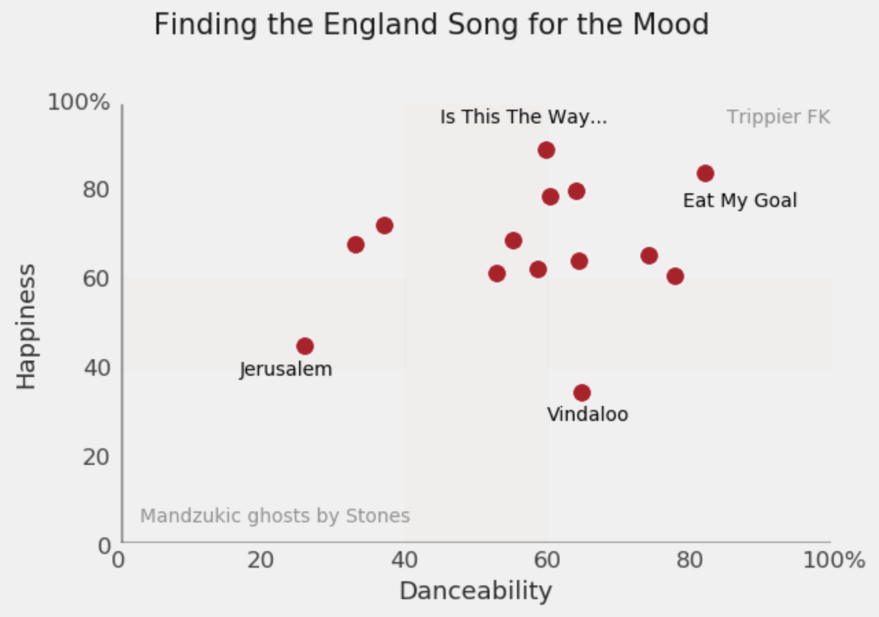
And now we have a data source for matching England songs to the tournament mood. Want something danceable at a high energy? Eat My Goal. Sad and low energy? Jerusalem.
We can even use the dataframes .sort_values() functionality to do the lookup for us based on what we want to see:
dataframe.sort_values("Happiness", ascending = False).head(3)
Now we have the 3 happiest songs in the playlist ready to go, and tough to argue with any of these.
Of course, you’d be unlikely to take a Jupyter notebook down the pub, or to your nearest riot, so I’d recommend making a print out graphic to take with you.
#Set base style and size
plt.style.use('fivethirtyeight')
plt.figure(num=None, figsize=(6, 4), dpi=100)

#Set subtle St. George's Cross underneath, don't want to come across strong
rect = patches.Rectangle((0.4,0),0.2,1, color="red", alpha=0.01)
plt.gca().add_patch(rect)
rect2 = patches.Rectangle((0,0.4),0.4,0.2, color="red", alpha=0.01)
plt.gca().add_patch(rect2)
rect3 = patches.Rectangle((0.6,0.4),1,0.2, color="red", alpha=0.01)
plt.gca().add_patch(rect3)

#Plot data
ax = sns.scatterplot(x="Danceability", y="Happiness", data=dataframe,
                     s=100, color='#b50523')

#Set title
ax.text(x = 0.05, y = 1.15, s = "Finding the England Song for the Mood",
               fontsize = 15, alpha = 0.9)
#Set Annotations
ax.text(x = 0.79, y = 0.76, s = "Eat My Goal",
               fontsize = 10, alpha = 1)
ax.text(x = 0.17, y = 0.38, s = "Jerusalem",
               fontsize = 10, alpha = 1)
ax.text(x = 0.6, y = 0.28, s = "Vindaloo",
               fontsize = 10, alpha = 1)
ax.text(x = 0.45, y = 0.95, s = "Is This The Way...",
               fontsize = 10, alpha = 1)

#Set mood examples
ax.text(x = 0.85, y = 0.95, s = "Trippier FK",
               fontsize = 10, alpha = 0.4)
ax.text(x = 0.03, y = 0.05, s = "Mandzukic ghosts by Stones",
               fontsize = 10, alpha = 0.4)

#Remove grid and add axis lines
ax.grid(False)
ax.axhline(y=0.005, color='#414141', linewidth=1.5, alpha=.5)
ax.axvline(x=0.005, color='#414141', linewidth=1.5, alpha=.5)

#Set axis limits
ax.set(ylim=(0,1))
ax.set(xlim=(0,1))

#Set axis labels
ax.set_yticklabels(labels=['0', '20', '40', '60', '80','100%'], fontsize=12, color='#414141')
ax.set_xticklabels(labels=['0', '20', '40', '60', '80','100%'], fontsize=12, color='#414141')

#Set axis titles
plt.xlabel('Danceability', fontsize=13, color='#2a2a2b')
plt.ylabel('Happiness', fontsize=13, color='#2a2a2b')

#Plot
ax.plot()
In this tutorial, we have seen how we can navigate the Spotify API by using the Spotipy module. We have found out how we can get data about songs, and navigate a playlist to do this programatically for a group of tracks.
As for wider Python skills, we have practiced how to loop through items and store information about each one. We have then joined this up into a dataframe for analysis and visualisation.