

If you want to move past aggregate data on players and teams, you probably want to start looking at match event data. Obtaining this data can be difficult, and even when you get there, it is often in an XML file, rather than a table that you might be more comfortable with. This article will take you through parsing an Opta F24 XML file into a table containing the passes within a game.
Firstly, it is probably worth understanding what an XML file is. It is simply a text file structured to hold data. It uses things called tags to explain what bits of data it holds and organises them in a structure that makes it easy to understand and use elsewhere. If you have any experience with HTML, it is very similar. Here is a simple example showing how an XML file might look to send data about managerial changes:
<team name = "Manchester United">
    <manager name = "Jose Mourinho" start = "2016/05/27" end = "2018/12/18" />
    <manager name = "Ole Gunnar Solskjær" start = "2018/12/19" />
</team>
So here we have a hierarchy of team -> manager, with attributes within each data point such as team name or start date. Hopefully it is clear to see how this standardised method of sharing information might make it so much easier to use data in our work or share data with others – especially when data have different amounts of characteristics as we see above.
However, if we want to use lots of Python’s plotting and analysis capabilities, we will likely need this data in a table – and this is what we will work towards. We’ll take the following steps:
- Import modules
- Load our XML file
- Explore the Opta F24 XML structure
- Iterate through the match events and save pass data into lists
- Merge these lists together into a table
Once we get through all of these steps, we’ll have a nice table with which we can do loads of plotting and analysis with!
As a quick note, this Opta feed isn’t publicly available and is largely only found in clubs, analytics companies and media organisations. Manchester City and Opta briefly released a season’s worth of data from 2011-12, although FC Python unfortunately do not have this available.
Follow along and import the modules below to get started!
import csv
import xml.etree.ElementTree as et
import numpy as np
import pandas as pd
from datetime import datetime as dt
Now that we’re ready to go, the first thing that we need to do is import our XML file. The XML module that we added above makes this really simple. The two lines below will take an XML file and parse it into something that we could navigate just like we do with an object by using square brackets:
tree = et.ElementTree(file = "yourf24XMLfile.xml")
gameFile = tree.getroot()
Opening up the XML file in a text editor, we can see that the F24 file is structured similar to below:
<Container>
    <Game>
        <Event>
            <Event Qualifiers>
            </Event Qualifiers>
        </Event>
        ...
        <Event>
            <Event Qualifiers>
            </Event Qualifiers>
        </Event>
    </Game>
</Container>
So we have a container for all the data, then a game that holds each event. Within each event, there are attributes telling us about the event as well as qualifiers giving even more information about each events.
We will get around to making sense of the events, but let’s take a look at what information we are given about the game itself. We can do this with the ‘.attrib’ method from the XML module imported earlier. Let’s check out the attributes from the first entry into our XML file (the one containing the match events). We can do this by using square brackets to select aspecific entry:
gameFile[0].attrib
Awesome, we get loads of information about the match in a dictionary, where the data is laid out with a key, then the value. For example, we can see the team names and also their Opta IDs.
These match details could be useful if we were processing lots of events at the same time and needed to differentiate them. Let’s look at a quick example of formatting a string with the details found here:
#Print a string with the two teams, using %s and the attrib to dynamically fill the string
print ("{} vs {}".format(gameFile[0].attrib["home_team_name"], gameFile[0].attrib["away_team_name"]))
Moving onto match events, we saw in the structure of the file that the match events lie within the game details tags. Let’s use another square bracket to navigate to the first event:
gameFile[0][0].attrib
Looking through this, there is a lot to try and get our heads around. We can see that there are event keys like min, sec, x and y – these are quite easy to understand. But the values, like outcome: 1 and event_id: 1, don’t really make much sense by themselves. This is particularly important when it comes to teams, as we only have their ID and not their name. We’ll tidy that up soon.
This is because the Opta XML uses lots of IDs rather than names. You’ll need to find documentation from Opta (although versions of this can be Googled) to find out what all of them are. But first one’s free, and our event_id: 1 is pass – as you’d probably expect for the first event from the game.
You might also remember that our events contained qualifiers. Let’s again use square brackets to pull the first one out for the event above:
gameFile[0][0][0].attrib
We don’t need to know what this means, but it is useful to understand the structure of the file as we will be going on to iterate through each event and qualifier to turn it into a table for further analysis.
At its simplest, all we are going to do is loop through each of the events that we have identified above, identify the passes and take the details that we want from each. These details will go into different lists for different data categories (player, team, success, etc.). We will then put these lists into a table which is then ready for analysis, plotting or exporting.
Firstly though, I’d like to have my team names come through to make this a bit more readble, while than the team ID. The events only carry the team ID, so let’s create a dictionary that will allow us to later swap the ID for the team name:
team_dict = {gameFile[0].attrib["home_team_id"]: gameFile[0].attrib["home_team_name"],
            gameFile[0].attrib["away_team_id"]: gameFile[0].attrib["away_team_name"]}


print(team_dict)
For this tutorial, we’re simply going to take the x/y locations of the pass origin and destination, the time of the pass, the team and whether or not it was successful.
There’s so much more that we could take, such as the players, the pass length or any other details that you spot in the XML. If you’d like to pull those out too, doing so will make a great extension to this tutorial!
We’re going to start by creating the empty lists for our data:
#Create empty lists for the 8 columns we're collecting data for
x_origin = []
y_origin = []
x_destination = []
y_destination = []
outcome = []
minute = []
half = []
team = []
The main part of the tutorial sees us going event-by-event and adding our desired details only when the event is a pass. To do this, we will use a for loop on each event, and when the event is a pass (id = 1), we will append the correct attribute to our lists created above. Some of these details are hidden in the qualifiers, so we’ll also iterate over those to get the information needed there.
This tutorial probably isn’t the best place to go through the intricacies of the feed, so take a look at the docs if you’re interested.
Follow the code below with comments on each of the above steps:
#Iterate through each game in our file - we only have one
for game in gameFile:

    #Iterate through each event
    for event in game:

        #If the event is a pass (ID = 1)
        if event.attrib.get("type_id") == '1':

            #To the correct list, append the correct attribute using attrib.get()
            x_origin.append(event.attrib.get("x"))
            y_origin.append(event.attrib.get("y"))
            outcome.append(event.attrib.get("outcome"))
            minute.append(event.attrib.get("min"))
            half.append(event.attrib.get("period_id"))
            team.append(team_dict[event.attrib.get("team_id")])

            #Iterate through each qualifier
            for qualifier in event:

                #If the qualifier is relevant, append the information to the x or y destination lists
                if qualifier.attrib.get("qualifier_id") == "140":
                    x_destination.append(qualifier.attrib.get("value"))
                if qualifier.attrib.get("qualifier_id") == "141":
                    y_destination.append(qualifier.attrib.get("value"))
If this has worked correctly, we should have 8 lists populated. Let’s check out the minutes list:
print("The list is " + str(len(minute)) + " long and the 43rd entry is " + minute[42])
You can check out each list in more detail, but they should work just fine.
Our final task is to create a table for our data from our lists. To do this, we just need to create a list of our column headers, then assign the list to each one. We’ll then flip our table to make it long, rather than wide – just like you would want to see in a spreadsheet. Let’s take a look:
#Create a list of our 8 columns/lists
column_titles = ["team", "half", "min", "x_origin", "y_origin", "x_destination", "y_destination", "outcome"]

#Use pd.DataFrame to create our table, assign the data in the order of our columns and give it the column titles above
final_table = pd.DataFrame(data=[team, half, minute, x_origin, y_origin, x_destination, y_destination, outcome], index=column_titles)

#Transpose, or flip, the table. Otherwise, our table will run from left to right, rather than top to bottom
final_table = final_table.T

#Show us the top 5 rows of the table
final_table.head()
So this is great for passes, and the same logic would apply for shots, fouls or even all events at the same time – just expand on the above with the relevant IDs from the Opta docs. And analysts, if you’re still struggling to get it done, the emergency loan window is always open!
Now that we’ve taken a complex XML and parsed the passes into a table, there’s a number of things that we can do. We could put the table into a wider dataset, do some analysis of these passes, visualise straight away or just export our new table to a csv:
final_table.to_csv("pass_data.csv", index=False)
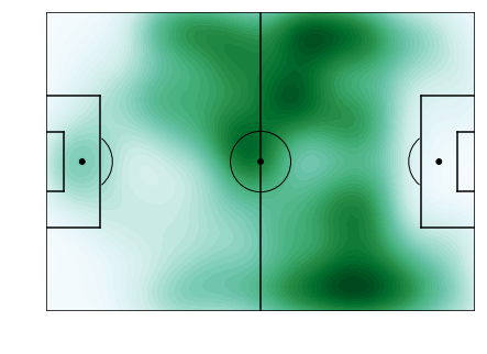
Heatmap – code taken from the FC Python tutorial
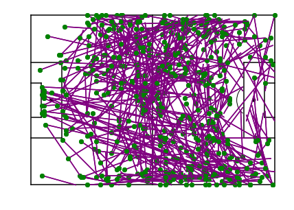
Passmap – full tutorial here.
Summary
In this tutorial, we’ve learned a bit about XML structures and the Opta F24 XML specifically. We have seen how to import them into Python and parse them into empty lists. With these now-full lists, we have gone on to pull these into a single table. From here, it is much easier to run our analysis, plot data or do whatever else we like. The further beauty of this comes in automating your analysis for future games and giving yourself hours of time each week.
Huge credit belongs to a number of sources that helped with this piece, including Imran Khan, FC R Stats and plenty of other posts that take a look at the feed.
With your newfound data from the Opta F24 XML, why not practice your visualisation skills with the data? Check out our collection of visualisation tutorials here.